Last time we began this series with the groundwork maths that we will need to get started in building out some machine learning algorithmns. In this post we are going to build out our first algorithm - linear regression.
Linear Regression - The Statistician’s Friend
When I began last time I mentioned we were going to try and cover a range of algorithms from pure statistics across to definitive machine learning methods, and highlight when that occurs. Linear regression is going to be our first algorithm and it is definitively on the statistics end of the spectrum - many high school courses will include this. We are going to start with linear regression because it allows us to understand at a more simplified level some of the mechanics that will become more important as we move into more complex algorithms. It is also a simple yet powerful algorithm that we will be extending in the future.
Some Data
| Number of Bedrooms | House price (£ rounded to nearest thousand) |
|---|---|
| 1 | 115 |
| 4 | 300 |
| 4 | 300 |
| 2 | 187 |
| 4 | 400 |
| 4 | 330 |
| 1 | 115 |
| 2 | 140 |
| 2 | 180 |
| 2 | 128 |
| 3 | 185 |
| 5 | 450 |
| 4 | 325 |
| 4 | 320 |
| 3 | 280 |
| 3 | 190 |
| 3 | 350 |
| 2 | 140 |
| 5 | 365 |
| 2 | 210 |
| 2 | 268 |
| 3 | 250 |
| 3 | 465 |
| 3 | 205 |
| 4 | 230 |
This is a set of data on house prices using the first results page from a UK house price website in a random area of the country.
We can plot the data of net spend against average position as follows
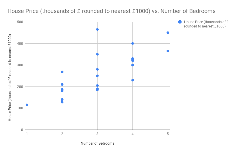
What we have here is a linear dataset, 2 variables (net spend and average position) that we believe to be connected by some correlation. We are going to avoid the correlation vs causation argument here and discuss that at a later date, but with this dataset we want to ascertain that if I were an property developer looking to build a set of 3 bedroom homes in this area, what would I expect to put them on the market for?
More Maths
Linear Regression works by looking at all of our data and plotting a line of the form:
[y = b_1 x + b_0]
where b1 is the Pearson Correlation Coefficient and b0 is the point at which our line intercepts the axis, also called our bias because we add this to manipulate and offset every prediction we make. “Correlation Coefficient” is maths terminology for scaling factor in the relationship. For example, let’s say you pay tax at 20% of your income. That means for every £1 you earn you get 80p, so the scaling factor - or coefficient - is 0.8
An Aside on Gradient Descent
A few people who are a bit more savvy with the world of ML and associated algorithms are probably now wondering “where is your gradient descent?” Great question! Because we have a very simple structure here we are going to use some regular statistical tools. You know I mentioned expanding in the future, well that is where we are going - you will just have to be patient.
Calculating Our Values
The Pearson Correlation Coefficient can be calculated for us as follows:
[r_{xy} = b_1 = \frac{1}{n - 1} \sum\limits_{i=1}^n \left(\frac{x_i - \bar{x}}{s_x}\right)\left(\frac{y_i - \bar{y}}{s_y}\right)]
Firstly, rxy is notation used in a lot of maths literature so I wanted to share it in case you see it elsewhere, but it is our correlation coefficient b1. We have seen almost everything here before, summing over all of our x values (net spend) and summing over all our y values (average position) along with the mean of x and mean of y (with the bars above them). sx and sy are shorthand for “the standard deviation of dataset x” (or respectively y) which again we covered in the last post. So everything here is pretty straightforward for us!
How do we calculate our b0? Well doing some simple algebra gives:
[b_0 = y - b_1 x]
(to do this, take b0x away from both sides of the equation we have) If we put inb to x and y the mean values for our set of x and y, we get the expected intercept.
Apex Time
Impressively, I have managed to get through almost one and a half blog posts titled “AI For Salesforce Developers” without writing a single line of Apex, well now let’s make the rubber hit the road! All the code (and some for future posts) is shared on Github. I will spend time here focussing on the Linear Regression class as it is what we care about. Separately I will add another post about the Matrix and Math classes.
Our Linear Regression class looks like this:
public with sharing class LinearRegression {

	private Double coefficient {get; private set;}
	private Double intercept {get; private set;}

	private List<Double> x_train {get; private set;}
	private List<Double> y_train {get; private set;}

	public LinearRegression(List<Double> x_data, List<Double> y_data) {
		x_train = x_data;
		y_train = y_data;
	}

	public void train() {
		Double mean_x = MathUtil.mean(x_train);
		Double mean_y = MathUtil.mean(y_train);
		coefficient = MathUtil.pearsonCorrelation(x_train, y_train);
		intercept = mean_y - coefficient*mean_x;
	}

	public Double predict(Double value) {
		return intercept + coefficient*value;
	}

	public Double rootMeanSquaredError() {
		List<Double> predictions = new List<Double>();
		Integer num_items = x_train.size();
		for(Integer i = 0; i < num_items; i++) {
			predictions.add(predict(x_train[i]));
		}

		List<Double> squaredErrors = new List<Double>();
		for(Integer i = 0; i < num_items; i++) {
			squaredErrors.add(Math.pow(predictions[i] - y_train[i], 2));
		}

		return MathUtil.mean(squaredErrors);
	}
}
We have an initialisation that takes in our x and y values, a train method that creates our intercept and coefficient, and a predict method to predict a value. We also have a rootMeanSquaredError function that we are going to use to give us an indication of the error in the data.
Run the Code! Make Some Predictions!
So let’s use this code and make some predictions. Run the following in Execute Anonymous:
List<Double> numBedrooms = new List<Double>{1,4,4,2,4,4,1,2,2,2,3,5,4,4,3,3,3,2,5,2,2,3,3,3,4};
List<Double> housePrice = new List<Double>{115,300,300,187,400,330,115,140,180,128,185,450,325,320,280,190,350,140,365,210,268,250,465,205,230};

LinearRegression linReg = new LinearRegression(numBedrooms, housePrice);
linReg.train();
System.debug('RMSE:' + linreg.rootMeanSquaredError());
System.debug('3 bedroom houses should be on sale for :' + linreg.predict(3));
Running this and reviewing our logs shows:
RMSE:9872.59041781244
3 bedroom houses should be on sale for :257.12
So £257,000 is the prediction, which if we look at the graph from above would seem about right. I say “seem about right” because part of reviewing your results should always be a use of your intuition given the knowledge of the dataset. If you know the dataset well and it “seems correct” then it probably is. Our common sense here would say that looking at the other prices that is in the correct area. If it seemed incorrect, it could be that it is, or in a dataset that is more complicated, with a larger number of features, it could be that there is a new insight we were not aware of previously and should investigate further with real world testing.
To quote Rick Sanchez (Rick from Rick and Morty):
Sometimes science is more art than science, Morty. Lot of people don’t get that.
We also see that the error is 9000 which is pretty large. This indicates that there is a fairly large degree of error in our predictions, and again looking at our dataset and predictions, this is understandable. Some reasons behind this could be:
- Lack of data. We are using a small sample size here, what would this look like with a much bigger data set?
- Lack of features. We are basing the price of a house purely upon the number of bedrooms whereas square foot space and location are also likely to be large factors.
Again, we have to be aware of all these things when generating a model - yes we can see how good it can be but we must also be aware of and communicate any limitations we can forsee in its setup. If we placed a one bedroom penthouse on this list it would likely skew the data wildly.
Summary
Congratulations! You have worked through your first algorithm and made a prediction based upon the data you have. This basic setup could be used for all manner of use cases, but becomes much more powerful when we add additional features.
The next post is going to be a summary of the rest of the Apex we have setup ready in the org and I will also find a good test dataset and load it into the repo as well for future use. From there we are going to rework this algorithm using gradient descent, update the model to use multiple parameters, and then move on to other types of algorithm. If you have any feedback on the series and the plan then let me know on Twitter.